These are some notes I took for the Microsoft exam 70-761: Querying Data with Transact-SQL, which is a part of MCSA: SQL 2016 Database Development.

This is for the syllabus as it was in May 2019. The syllabus might change in the future. I’ve mainly taken notes from the official documentation and the official exam book. I recommend getting the book to make sure you know everything that has to be known at the exam. I also recommend reading some of the articles on Erland Sommerskog’s web page, especially the articles on error handling.

Microsoft likes to ask questions on features that are new in the latest version of SQL Server. This is done to make sure people with an older version of the certification can’t pass without studying when going for the newest version of the certification. SQL Server 2016 introduced JSON and temporal tables, so make sure you know those topics very well.

Manage data with Transact-SQL
Query data with advanced Transact-SQL components
Program databases by using Transact-SQL
Not part of the official syllabus
- Spatial data
- Cursors

Manage data with Transact-SQL (40–45%)

Create Transact-SQL SELECT queries

Syllabus

Identify proper SELECT query structure, write specific queries to satisfy business requirements, construct results from multiple queries using set operators, distinguish between UNION and UNION ALL behaviour, identify the query that would return expected results based on provided table structure and/or data

SELECT in general

Official documentation

Basic examples:

-- Generic SELECT
SELECT * FROM accounts

-- SELECT with WHERE clause
SELECT * FROM accounts WHERE accountId = 12

-- SELECT with WHERE clause containing AND:
SELECT * FROM customers WHERE city = 'New York City' AND gender = 'Male'

-- SELECT with WHERE clause containing OR:
SELECT * FROM customers WHERE city = 'New York City' OR city = 'Boston'

-- SELECT with WHERE clause checking for not null:
SELECT * FROM customers WHERE city IS NOT NULL

-- SELECT that only gets certain columns
SELECT firstName, lastName FROM customers

-- SELECT with alias for columns
SELECT firstName AS [First name], lastName AS [Last name] FROM customers

-- or
SELECT firstName AS 'First name', lastName AS 'Last name' FROM customers

-- Get only distinct elements
SELECT DISTINCT lastName FROM customers

LIKE:

Search with LIKE:

SELECT * FROM customers WHERE lastName LIKE '%son'

Wildcards:

Wildcard	Description
`%`	Any string
`_`	Any single character
`[ABC]`	A single character, either A, B or C
`[A-R]`	A single character, in the range A to R
`[ABC]`	A single character, not A, B or C
`[^A-R]`	A single character, not in the range A to R

TOP:

Official documentation on TOP

Get TOP elements:

SELECT TOP (100) *
FROM customers
ORDER BY customerId

-- Or skip the parentheses (correct is with):
SELECT TOP 100 *
FROM customers
ORDER BY customerId

-- Get TOP percent elements:
SELECT TOP (10) PERCENT *
FROM customers
ORDER BY customerId

Amount of rows returned with PERCENT is rounded up.

ORDER BY should also be used when using TOP, otherwise the order is non-deterministic and pretty much like the data is stored on disk.

OFFSET and FETCH:

Official documentation on OFFSET and FETCH

SELECT *
FROM customers
ORDER BY customerId
OFFSET 50 ROWS FETCH NEXT 10 ROWS ONLY

ORDER BY is mandatory with OFFSET and FETCH. OFFSET is mandatory with FETCH.

OFFSET and FETCH are part of the SQL standard. TOP is not.

UNION and UNION ALL

Official documentation

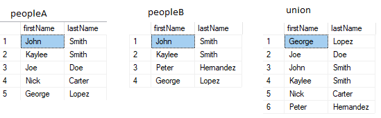
UNION is all rows in A and all rows in B. Distinct rows only.

SELECT firstName, lastName FROM peopleA
UNION
SELECT firstName, lastName FROM peopleB

Example of UNION

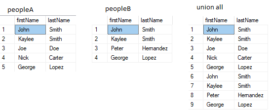
UNION ALL is all rows in A and all rows in B. Non-distinct rows are also returned.

SELECT firstName, lastName FROM peopleA
UNION ALL
SELECT firstName, lastName FROM peopleB

Example of UNION ALL

Number of columns must be the same in the two sets.
Column data type must be the same or compatible (implicitly convertible).

Difference between UNION and UNION ALL

Stack Overflow: What is the difference between UNION and UNION ALL?

Union is the union of two sets, e.g. two tables merged together. UNION will remove duplicates, while UNION ALL will not.

UNION ALL is faster as it doesn’t have to scan for duplicates.

INTERSECT

Official documentation

Finds rows that are common for both table A and B.

SELECT firstName, lastName FROM peopleA
INTERSECT
SELECT firstName, lastName FROM peopleB

Example of INTERSECT

Number of columns must be the same in the two sets.
Column data type must be the same or compatible (implicitly convertable).

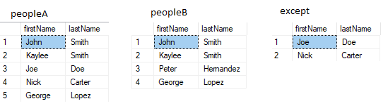
EXCEPT

Official documentation

Finds rows that are in A, but not in B.

SELECT firstName, lastName FROM peopleA
EXCEPT
SELECT firstName, lastName FROM peopleB

Example of EXCEPT 1

SELECT firstName, lastName FROM peopleB
EXCEPT
SELECT firstName, lastName FROM peopleA

Example of EXCEPT 2

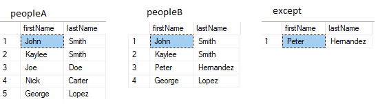
Number of columns must be the same in the two sets.
Column data type must be the same or compatible (implicitly convertable).

Special rules

Precedence order: parentheses, NOT, AND and then OR.
SQL Server doesn’t necessarily go left-to-right in WHERE clause predicates.
Thus no short-circuiting in WHERE clause predicates.
Keyed-in order:
- SELECT
- FROM
- WHERE
- GROUP BY
- HAVING
- ORDER BY
Phases of logic querying processing:
- FROM
- WHERE
- GROUP BY
- HAVING
- SELECT
- ORDER BY
  
  Because SELECT is processed after FROM, WHERE, etc. you can’t use column aliases made in SELECT in FROM, WHERE, etc.
When ORDER BY is used the result is no longer relational.

Query multiple tables by using joins

Syllabus

Write queries with join statements based on provided tables, data, and requirements; determine proper usage of INNER JOIN, LEFT/RIGHT/FULL OUTER JOIN, and CROSS JOIN; construct multiple JOIN operators using AND and OR; determine the correct results when presented with multi-table SELECT statements and source data; write queries with NULLs on joins

Joins

Official documentation

These tables are used in this chapter:

CREATE TABLE men (
    Id           INT           IDENTITY(1,1)  NOT NULL
  , firstName    VARCHAR(200)
  , lastName     VARCHAR(200)
  , marriedToId  INT
)

CREATE TABLE women (
    Id           INT           IDENTITY(1,1)  NOT NULL
  , firstName    VARCHAR(200)
  , lastName     VARCHAR(200)
  , marriedToId  INT
)

INSERT INTO men (firstName, lastName, marriedToId) VALUES
    ('Samuel', 'McDonald' , 2   )
  , ('Jack'  , 'Lipinski' , 1   )
  , ('Roger' , 'Pierce'   , NULL)
  , ('Travis', 'Danielson', NULL)

INSERT INTO women (firstName, lastName, marriedToId) VALUES
    ('Lisa'   , 'Samson'  , 2   )
  , ('Linda'  , 'Windsor' , 1   )
  , ('Beyonce', 'Corleone', NULL)

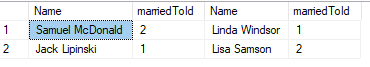
INNER JOIN

Inner joins will only match if there are values in both left and right tables.

Example:

SELECT
    m.firstName + ' ' + m.lastName AS Name
  , m.marriedToId
  , w.firstName + ' ' + w.lastName AS Name
  , w.marriedToId
FROM men m
  INNER JOIN women w ON m.Id = w.marriedToId

INNER JOIN query output

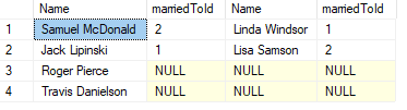
LEFT JOIN

Left join will return everything in the left table, even if there are no matches in the right table.

SELECT
    m.firstName + ' ' + m.lastName AS Name
  , m.marriedToId
  , w.firstName + ' ' + w.lastName AS Name
  , w.marriedToId
FROM men m
  LEFT JOIN women w ON m.Id = w.marriedToId

LEFT JOIN query output

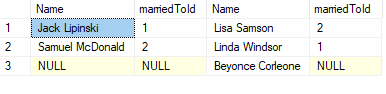
RIGHT JOIN

A right join is like a left join, but with left and right tables switched.

SELECT
    m.firstName + ' ' + m.lastName AS Name
  , m.marriedToId
  , w.firstName + ' ' + w.lastName AS Name
  , w.marriedToId
FROM men m
  RIGHT JOIN women w ON m.Id = w.marriedToId

RIGHT JOIN query output

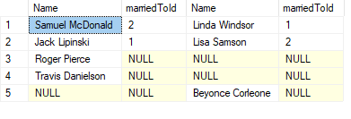
FULL OUTER JOIN

Full outer joins will return everything in both the left and right tables.

SELECT
    m.firstName + ' ' + m.lastName AS Name
  , m.marriedToId
  , w.firstName + ' ' + w.lastName AS Name
  , w.marriedToId
FROM men m
  FULL JOIN women w ON m.Id = w.marriedToId

FULL OUTER JOIN query output

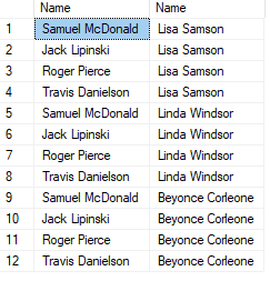
CROSS JOIN

Cross join returns the Cartesian product of left and right table. That is all the possible combinations of selected rows in left and right.

Example:

SELECT
    m.firstName + ' ' + m.lastName AS Name
  , w.firstName + ' ' + w.lastName AS Name
FROM men m
  CROSS JOIN women w

CROSS JOIN query output

Query with NULL on joins

Rows that have null on one or more of the joined-on keys will be filtered out when using inner joins. To preserve the row, an outer join must be used.

When joining on multiple keys, where one or more of the keys can be null, we have to handle the nulls in the join. A naive way of handling the null could be like this:

CREATE TABLE customers (
    Id         INT            IDENTITY(1,1)   NOT NULL
  , firstName  VARCHAR(200)
  , lastName   VARCHAR(200)
  , SSN        VARCHAR(20)
)

INSERT INTO customers (firstName, lastName) VALUES
    ('Alex' , 'Golding'  )
  , ('Pablo', 'Fernandez')

INSERT INTO customers (SSN) VALUES
    ('1234567892')
  , ('1234567893')

CREATE TABLE accounts (
    Id         INT            IDENTITY(1,1)   NOT NULL
  , firstName  VARCHAR(200)
  , lastName   VARCHAR(200)
  , SSN        VARCHAR(20)
)

INSERT INTO accounts (firstName, lastName) VALUES
    ('Alex' , 'Golding'  )
  , ('Pablo', 'Fernandez')

INSERT INTO accounts (SSN) VALUES
    ('1234567892')
  , ('1234567893')

SELECT *
FROM customers c
  INNER JOIN accounts a ON
          ISNULL(c.firstName, 'N/A') = ISNULL(a.firstName, 'N/A')
      AND ISNULL(c.lastName,  'N/A') = ISNULL(a.lastName,  'N/A')
      AND ISNULL(c.SSN,       'N/A') = ISNULL(a.SSN,       'N/A')

The problem with this is that a column is being manipulated, which also means that the order of the result no longer is preserved. This will also affect the performance. A better solution for handling the null values would be:

SELECT *
FROM customers c
  INNER JOIN accounts a ON
      (c.firstName = a.firstName
        OR (c.firstName IS NULL AND a.firstName IS NULL))
      AND (c.lastName = a.lastName
        OR (c.lastName IS NULL AND a.lastName IS NULL))
      AND (c.SSN = a.SSN
        OR (c.SSN IS NULL AND a.SSN IS NULL))

According to the exam book, an even better solution could be:

SELECT *
FROM customers c
    INNER JOIN accounts a ON
    EXISTS (SELECT c.firstName, c.lastName, c.SSN
            INTERSECT
            SELECT a.firstName, a.lastName, a.SSN)

Implement functions and aggregate data

Syllabus

Construct queries using scalar-valued and table-valued functions; identify the impact of function usage to query performance and WHERE clause sargability; identify the differences between deterministic and non-deterministic functions; use built-in aggregate functions; use arithmetic functions, date-related functions, and system functions

Search Argument Able

A WHERE clause is sargable when the query engine can use index seek rather than scan. That means a query that is made in such a way that it uses a created index. This makes the query much faster than a query that doesn’t use a created index, because these queries have to go through the entire table to find matches. We should therefore strive to make queries sargable.

The following can make queries non-sargable:

Manipulation of filtered columns in most cases.
Functions that have a column as argument, except in certain circumstances.
LIKE clauses like this: '%test%'. 'test%' would be OK.
Using ISNULL() in the WHERE clause.
Using arithmetic on the filtered column.

Exceptions:

CAST(datetime AS DATE) = '20190505', when datetime is indexed and of datetime type. SQL Server can convert this to an interval.

Differences between deterministic and non-deterministic functions

Official documentation

Deterministic functions always return the same given a specific input and state of database. E.g. AVG().
Non-deterministic functions can return different values each time they are called, even though the input and state of database is the same. E.g. GETDATE().
Determinism of a function determine the ability of SQL Server to index the result of a function.
A clustered index cannot be created on a view that uses a non-deterministic function.
Certain non-deterministic functions can be used in indexed views if they are used in a deterministic matter. E.g. RAND() when a seed is specified.

Type conversion functions

Official documentation

T-SQL has two main functions for conversion purposes: CAST() and CONVERT(). CONVERT() is T-SQL only, while CAST() is a part of the SQL standard.

Example:

CAST syntax:

SELECT CAST('123' AS INT)    -- outputs 123

CONVERT syntax without style:

SELECT CONVERT(INT, '123')   -- outputs 123

CONVERT syntax with style:

SELECT CONVERT(VARCHAR, GETDATE(), 103)   -- outputs '05/05/2019'

There are also a couple of other type conversion functions that can be used:

PARSE (alternative to CAST):

SELECT PARSE('01/05/2019' AS DATE USING 'en-US')  -- outputs 2019-01-05
SELECT PARSE('01/05/2019' AS DATE USING 'no-NO')  -- outputs 2019-05-01

FORMAT (alternative to CONVERT):

SELECT FORMAT(GETDATE(), 'yyyy-MM-dd')  -- outputs 2019-05-05

PARSE and FORMAT are slow. Try to use CAST and CONVERT instead.

TRY_CAST, TRY_CONVERT and TRY_PARSE will return NULL if they fail to convert:

SELECT PARSE('40/05/2019' AS DATE USING 'en-US')
-- exception: Error converting string value '40/05/2019'
-- into data type date using culture 'en-US'.

SELECT TRY_PARSE('40/05/2019' AS DATE USING 'en-US')  -- outputs NULL

Built-in aggregate functions

Official documentation

“An aggregate function performs a calculation on a set of values, and returns a single value.”

CREATE TABLE people (
    Id    INT            IDENTITY(1,1)    NOT NULL
  , name  VARCHAR(100)
  , age   INT
)

INSERT INTO people (name, age) VALUES
    ('John Smith',      27)
  , ('Kaylee Smith',    26)
  , ('Peter Hernandez', 52)
  , ('George Lopez',    77)

Not needing GROUP BY:

SELECT COUNT(*)    FROM people -- outputs 4
SELECT AVG(age)    FROM people -- outputs 45
SELECT MIN(age)    FROM people -- outputs 26
SELECT MAX(age)    FROM people -- outputs 77
SELECT SUM(age)    FROM people -- outputs 182
SELECT VAR(age)    FROM people -- outputs 585.666... - variance for subset
SELECT VARP(age)   FROM people -- outputs 439.25     - variance for population
SELECT STDEV(age)  FROM people -- outputs 24.200...  - std dev for subset
SELECT STDEVP(age) FROM people -- outputs 20.958...  - std dev for population

All functions ignore NULL, except COUNT.

Arithmetic functions

Operators:

+: addition
-: subtraction
*: multiplication
/: division
%: modulo

Precedence is like in ordinary mathematics.

Integer division gives an integer as result:

SELECT 25 / 2		-- output is 12

It truncates.

Character functions

String concatenation can be done with either + or with the CONCAT() function.

Example:

SELECT 
  firstName + ' ' + lastName AS Name
FROM customers

SELECT 
  CONCAT(firstName, ' ', lastName) AS Name
FROM customers

When either operand to + is NULL, the entire value becomes NULL. CONCAT() will use an empty string when it encounters NULL.

SUBSTRING() is used to extract a string from another string.

Example:

SELECT SUBSTRING('Lauren Best', 2, 5)  -- outputs 'auren'

LEFT() and RIGHT() extracts string from left and right side of the string.

Example:

SELECT LEFT ('Lauren Best', 6)  -- outputs 'Lauren'
SELECT RIGHT('Lauren Best', 4)  -- outputs 'Best'

CHARINDEX() looks for the first occurence of a given substring in a string.

Example:

SELECT CHARINDEX('test', 'this is a test')  -- outputs 11

PATINDEX() looks for the first occurence of a given substring in a string, but uses pattern expressions.

Example:

SELECT PATINDEX('%test%', 'this is a test') -- outputs 11
SELECT PATINDEX('%t__s%', 'This is a test') -- outputs 1

LEN() returns the character length of a string.

Example:

DECLARE @str VARCHAR(20) = 'test'

SELECT LEN(@str)  -- outputs 4

Trailing spaces are not counted.

REPLACE() replaces a substring in a string with a new substring.

Example:

SELECT REPLACE('2019-05-18', '-', '/')  -- outputs '2019/05/18'

REPLICATE() replicates a string a given number of times.

Example:

SELECT REPLICATE('test ', 2)  -- outputs 'test test '

STUFF() removes a given number of characters in a string and then inserts a new substring in the same place.

Example:

SELECT STUFF('test', 1, 2, 'a')  -- outputs 'ast'

UPPER(), LOWER(), LTRIM() and RTRIM() can be used to format strings.

Example:

SELECT LOWER('Test')      -- outputs 'test'
SELECT UPPER('Test')      -- outputs 'TEST'
SELECT LTRIM('  Test  ')  -- outputs 'Test  '
SELECT RTRIM('  Test  ')  -- outputs '  Test'

STRING_SPLIT() can be used to split a string given a delimiter.

Example:

SELECT value FROM STRING_SPLIT('123;456;789', ';')

/* Output is
1   123
2   456
3   789
*/

Official documentation

SQL Server has several types for storing and representing date and time:

DATE
TIME
SMALLDATETIME
DATETIME
DATETIME2
DATETIMEOFFSET

DATETIME2 has higher accuracy than DATETIME, which has higher accuracy than SMALLDATETIME. DATE is only for date and TIME is only for time. DATETIMEOFFSET is time-zone aware.

SQL Server has the following date and time functions:

GETDATE() returns the current date as a DATETIME.
CURRENT_TIMESTAMP returns the same as GETDATE(), but is a part of the SQL Standard.
SYSDATETIME() and SYSDATETIMEOFFSET() returns the current date in DATETIME2 and DATETIMEOFFSET format.
GETUTCDATE() returns the current date and time in UTC as a DATETIME.
SYSUTCDATETIME() returns the current date and time in UTC as a DATETIME2.

To get the current date, use CAST(SYSDATETIME() AS DATE).

DATEPART() can be used to extract year, month or day from a date.

Example:

DECLARE @date VARCHAR(8) = '20190518'
SELECT DATEPART(year, @date), DATEPART(month, @date), DATEPART(day, @date)
-- outputs 2019, 5, 18

DATENAME() can be used to extract the names of the date parts from a date.

Example:

DECLARE @date VARCHAR(8) = '20190518'
SELECT DATENAME(month, @date), DATENAME(weekday, @date)
-- outputs May, Saturday

The following functions can be used to create datetime values from numeric parts:

DATEFROMPARTS()
DATETIMEFROMPARTS()
DATETIME2FROMPARTS()
DATETIMEOFFSETFROMPARTS()
SMALLDATETIMEFROMPARTS()
TIMEFROMPARTS()

Example:

SELECT DATETIMEFROMPARTS(2019, 05, 18, 0, 0, 0, 0)
-- output is 2019-05-18 00:00:00

EOMONTH() can be used to find the date that is the end of the month for a given date.

Example:

SELECT EOMONTH(DATEFROMPARTS(2019, 05, 18))
-- output is 2019-05-31

DATEADD() is used to add a year, month or day to a given date.

Example:

SELECT DATEADD(month, 2, '2019-05-18')
-- output is 2019-07-18 00:00:00

DATEDIFF() is used to find the difference between two dates.

Example:

SELECT DATEDIFF(day, '2019-05-01', '2019-05-18')
-- output is 17

DATEDIFF() only looks at the part in the first argument. The rest are ignored.

SWITCHOFFSET() is used to adjust the time zone of a value that has type DATETIMEOFFSET.

Example:

DECLARE @dt DATETIMEOFFSET = '2019-05-18 06:00:00 -07:00'
SET @dt = SWITCHOFFSET(@dt, '-01:00')

PRINT @dt   -- output is 2019-05-18 12:00:00.0000000 -01:00

To convert a datetime that doesn’t have time zone to one that does, we can use the function TODATETIMEOFFSET().

Example:

DECLARE @dt  DATETIME = '2019-05-18 06:00:00'
DECLARE @dto DATETIMEOFFSET

SET @dto = TODATETIMEOFFSET(@dt, '+02:00')

PRINT @dto  -- output is 2019-05-18 06:00:00.0000000 +02:00

AT TIME ZONE can be used to make datetimes aware of daylight savings.

Official documentation for AT TIME ZONE

When AT TIME ZONE is used on a value without time zone, it does not adjust the date and time.

Example:

DECLARE @dt DATETIME2 = '2019-05-18 06:00:00'
SELECT @dt AT TIME ZONE 'Central European Standard Time'
-- output is 2019-05-18 06:00:00 +02:00

When AT TIME ZONE is used on a value with time zone, it will also adjust the time and date.

Example:

DECLARE @dt DATETIMEOFFSET = '2019-05-18 06:00:00 +00:00'
SELECT @dt AT TIME ZONE 'Central European Standard Time'
-- output is 2019-05-18 08:00:00 +02:00

Case expressions

Official documentation

CASE can be used to apply conditional logic. CASE has two forms: the simple form and the searched form.

Example with simple form:

SELECT
      firstName
    , lastName
    , age
    , CASE SIGN(age - 18)
        WHEN 1 THEN 'Overage'
        WHEN 0 THEN 'Overage'
        ELSE 'Underage'
      END AS ageStatus
FROM customers

It compares the input to multiple possible scalars.

Example with searched form:

SELECT
      firstName
    , lastName
    , age
    , CASE
        WHEN age >= 18 THEN 'Overage'
        ELSE 'Underage'
      END AS ageStatus
FROM customers

Searched form uses predicates in the WHEN clauses.

System functions

Official documentation

@@ROWCOUNT: returns number of rows affected by last statement as INT.
@@ROWCOUNT_BIG: returns number of rows affected by last statement as BIGINT.

COMPRESS() compresses string with gzip:

INSERT INTO customers (name, customer_data)
  VALUES('John Smith', COMPRESS(@data))

DECOMPRESS() decompresses data that was compressed with COMPRESS():

SELECT
  name,
  CAST(DECOMPRESS(customer_data) AS NVARCHAR(MAX)) AS customer_data
FROM customers

COMPRESS() and DECOMPRESS() requires SQL Server 2016.

CONTEXT_INFO can be used to pass parameters to modules that don’t support parameters, such as triggers.

CONTEXT_INFO: VARBINARY(128)

Storing in CONTEXT_INFO:

DECLARE @context_info VARBINARY(128) = CAST('test' AS VARBINARY(128))
SET CONTEXT_INFO @context_info

Reading from CONTEXT_INFO:

SELECT CAST(CONTEXT_INFO() AS VARCHAR(128))

There is only one context info per session.

SESSION_CONTEXT can also be used to pass parameters to modules that don’t support parameters. SESSION_CONTEXT acts as a key-value store rather than a single binary string.

Storing in SESSION_CONTEXT:

EXEC sys.sp_set_session_context
    @key   = N'environment'
  , @value = N'test'

Reading from SESSION_CONTEXT:

SELECT SESSION_CONTEXT(N'environment') AS environment

SESSION_CONTEXT is available from SQL Server 2016.

NEWID() can be used to generate GUIDs.

Example:

SELECT NEWID()  -- outputs A182DF6A-80AD-4F23-870F-B0BC6973D1C2

NEWSEQUENTIALID() can be used to generate always-increasing GUIDs. Can only be used in default constraints.

SCOPE_IDENTITY() returns the last id inserted into a table with an identity column. It has one of these scopes:

stored procedure
trigger
function
batch

This is unlike @@IDENTITY, which is not limited to a scope.

Modify data

Syllabus

Write INSERT, UPDATE, and DELETE statements; determine which statements can be used to load data to a table based on its structure and constraints; construct Data Manipulation Language (DML) statements using the OUTPUT statement; determine the results of Data Definition Language (DDL) statements on supplied tables and data

INSERT

Official documentation

There are four different ways to insert rows in tables:

INSERT VALUES
INSERT SELECT
INSERT EXEC
SELECT INTO

Example with INSERT VALUES:

INSERT INTO customers (firstName, lastName) VALUES
	('John', 'Smith'),
	('Mary', 'Lietchstad')

If a column does not get a value set, it must have a DEFAULT constraint, have an IDENTITY property or be able to store NULL.
Use SET IDENTITY_INSERT dbo.customers ON to manually specify values for columns with the IDENTITY property. Use SET IDENTITY_INSERT dbo.customers OFF afterwards.

Example with INSERT SELECT:

INSERT INTO customers (firstName, lastName)
  SELECT firstName, lastName FROM newCustomers

Example with INSERT EXEC:

INSERT INTO customers (firstName, lastName)
  EXEC CreateNewCustomer @firstName = 'Peter', @lastName = 'Anderson'

Example with SELECT INTO:

SELECT firstName, lastName
INTO export_to_DWH
FROM customers c
  INNER JOIN accounts c.account_id = a.id

Definition is taken from the result of the query.
Indexes, constraints, triggers and permissions are not copied to the new table.

UPDATE

Official documentation

Examples:

Ordinary:

UPDATE customers
SET lastName = 'Whitaker'
WHERE id = 3

Compound assignment:

UPDATE customers
SET age += 1
WHERE id = 1

With join:

UPDATE c
SET c.status = 'inactive'
FROM customers c
  INNER JOIN accounts a ON c.id = a.customer_id
WHERE a.status = 'inactive'

Using joins in UPDATE is T-SQL.

With variable:

DECLARE @age INT

UPDATE customers
SET @age = age += 1
WHERE id = 1

DELETE

Official documentation

Example:

DELETE FROM customers
WHERE lastName = 'Smithers'

Or everything in the customers table:

DELETE FROM customers

With join:

DELETE FROM c
  FROM customers c
  INNER JOIN accounts a ON c.id = a.customer_id
WHERE a.status = 'inactive'

Ids are not reused after a row is deleted with DELETE.
DELETE is logged.

Truncating a table:

TRUNCATE TABLE customers

The identity columns will be reset, e.g. id will start at 1 again.
Truncating uses optimized logging and therefore faster than deleting.

MERGE

Official documentation

MERGE can be used to merge one table into another.

Example:

CREATE TABLE customers
(
    Id           INT            IDENTITY(1,1)    NOT NULL
  , firstName    VARCHAR(100)
  , lastName     VARCHAR(100)
  , age          INT
)

CREATE TABLE newCustomers
(
    Id           INT            IDENTITY(1,1)    NOT NULL
  , firstName    VARCHAR(100)
  , lastName     VARCHAR(100)
  , age          INT
)

INSERT INTO customers    (firstName, lastName, age) VALUES
    ('John', 'Smith',  45)
  , ('Joe',  'Schmoe', 11)
  , ('Mary', 'Christ', 73)

INSERT INTO newCustomers (firstName, lastName, age) VALUES
    ('John',  'Smith',    46)
  , ('Alan',  'Goldberg', 23)
  , ('Sue',   'Hotz',     66)
  , ('Karen', 'Deville',  32)

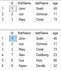
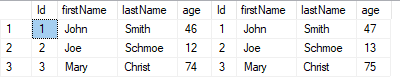
SELECT * FROM customers

MERGE INTO customers AS trg
USING newCustomers   AS src
ON trg.firstName = src.firstName AND trg.lastName = src.lastName
WHEN MATCHED THEN
  UPDATE SET
      firstName = src.firstName
    , lastName  = src.lastName
    , age       = src.age
WHEN NOT MATCHED THEN
  INSERT (firstName, lastName, age)
  VALUES (src.firstName, src.lastName, src.age);

SELECT * FROM customers

Example of MERGE

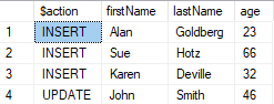
The OUTPUT clause is often used with MERGE:

MERGE INTO customers AS trg
USING newCustomers   AS src
ON trg.firstName = src.firstName AND trg.lastName = src.lastName
WHEN MATCHED THEN
  UPDATE SET
      firstName = src.firstName
    , lastName  = src.lastName
    , age       = src.age
WHEN NOT MATCHED THEN
  INSERT (firstName, lastName, age)
  VALUES (src.firstName, src.lastName, src.age)
OUTPUT $action, INSERTED.firstName, INSERTED.lastName, INSERTED.age;

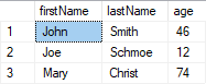
Example of MERGE with OUTPUT

OUTPUT

Official documentation

OUTPUT is used to output the result of an expression that affects rows. The table INSERTED will contain the new values and DELETED will contain the old values.

Example with only updated values:

UPDATE customers SET age += 1
OUTPUT INSERTED.firstName, INSERTED.lastName, INSERTED.age;

OUTPUT with updated values only

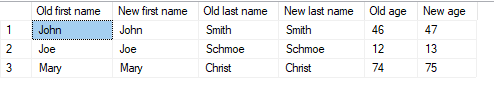
Example with old and new values:

UPDATE customers SET age += 1
OUTPUT DELETED.firstName AS 'Old first name', INSERTED.firstName AS 'New first name',
       DELETED.lastName  AS 'Old last name',  INSERTED.lastName  AS 'New last name',
       DELETED.age       AS 'Old age',        INSERTED.age       AS 'New age';

OUTPUT with both old and new values

Example with *:

UPDATE customers SET age += 1
OUTPUT DELETED.*, INSERTED.*

OUTPUT with both old and new values

Query data with advanced Transact-SQL components (30–35%)

Query data by using subqueries and APPLY

Syllabus

Determine the results of queries using subqueries and table joins, evaluate performance differences between table joins and correlated subqueries based on provided data and query plans, distinguish between the use of CROSS APPLY and OUTER APPLY, write APPLY statements that return a given data set based on supplied data

Subqueries

Subqueries are inner queries in an outer query.

A self-contained subquery does not have any dependency on the outer query. A subquery can return either a single value or a table of values. When a subquery returns a table of values it’s called a table expression. A subquery that returns a single value can be used in comparisons.

Example:

CREATE TABLE customers (
    Id          INT           IDENTITY(1,1)  NOT NULL
  , firstName   VARCHAR(200)
  , lastName    VARCHAR(200)
  , age         INT
)

INSERT INTO dbo.customers (firstName, lastName, age) VALUES
    ('John'  , 'Smith'     , 77)
  , ('Anette', 'DeLorean'  , 43)
  , ('Julian', 'Washington', 52)
  , ('Ariana', 'Brown'     , 55)

SELECT *
FROM customers
WHERE age > 10 + (SELECT min(age) FROM customers)

/* Outputs:
1   John     Smith   77
4   Ariana   Brown   55
*/

The query fails if the inner query returns multiple rows, and a scalar is expected.
IN can be used if the inner query returns multiple rows.

The following predicates can be used with the subquery: ALL, ANY and SOME.

Example:

SELECT *
FROM customers
WHERE age > ALL (SELECT age FROM customers WHERE age BETWEEN 43 AND 56)

/* Outputs:
1   John   Smith   77
*/

SELECT *
FROM customers
WHERE age = ANY (SELECT age FROM customers WHERE age BETWEEN 43 AND 56)

/* Outputs:
2   Anette   DeLorean    43
3   Julian   Washington  52
4   Ariana   Brown       55
*/

SELECT *
FROM customers
WHERE age = SOME (SELECT age FROM customers WHERE age BETWEEN 43 AND 56)

/* Outputs:
2   Anette   DeLorean    43
3   Julian   Washington  52
4   Ariana   Brown       55
*/

ALL returns true if all values returned from the subquery are equal to the left side of the expression.
ANY or SOME will return true if at least one of the values returned from the subquery are equal to the left side of the expression.

A correlated subquery has a dependency on the outer query.

Example:

CREATE TABLE customers (
    Id          INT           IDENTITY(1,1)  NOT NULL
  , firstName   VARCHAR(200)
  , lastName    VARCHAR(200)
  , age         INT
)

CREATE TABLE accounts (
    Id         INT            IDENTITY(1,1)  NOT NULL
  , customerId INT
  , balance    MONEY
)

INSERT INTO dbo.customers (firstName, lastName, age) VALUES
    ('John'  , 'Smith'     , 77)
  , ('Anette', 'DeLorean'  , 43)

INSERT INTO dbo.accounts (customerId, balance) VALUES
    (1, 100)
  , (2, 50)

SELECT *
FROM customers c
WHERE EXISTS(
  SELECT 1
  FROM accounts a
  WHERE c.Id = a.customerId
)

/* Outputs:
1   John     Smith      77
2   Anette   DeLorean   43
*/

Subqueries vs joins

Joins are more efficient than subqueries in most cases. However, there are certain circumstances where subqueries are faster.

Example (two large and almost identical tables):

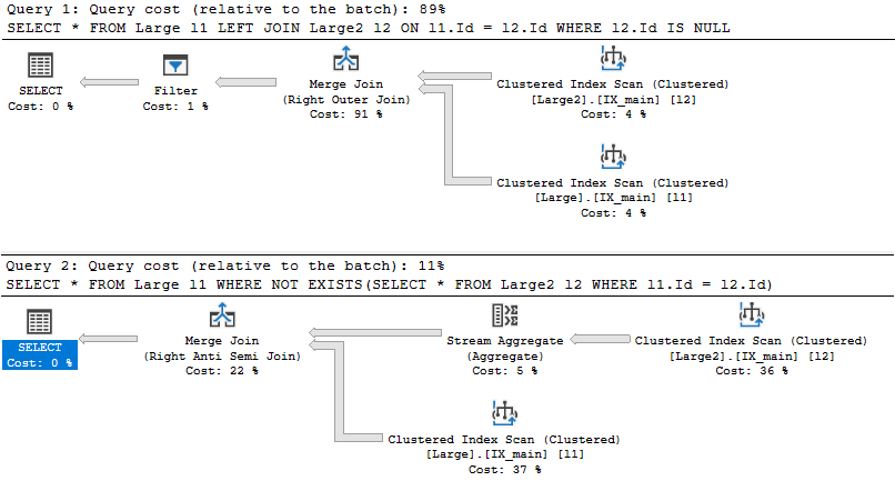
SELECT *
FROM Large l1
  LEFT JOIN Large2 l2 ON l1.Id = l2.Id
WHERE l2.Id IS NULL

SELECT *
FROM Large l1
WHERE NOT EXISTS(SELECT * FROM Large2 l2 WHERE l1.Id = l2.Id) 

These queries try to find rows in Large that are not in Large2. In this case, the subquery method will be faster. The inner query will return immediately when it finds a match in Large2. The join solution, however, will go through all the rows in Large2, and then later filter out unwanted rows with the WHERE clause.

The short-circuiting done in the subquery solution is called anti semi join optimization. This makes the subquery solution cost less than the join solution

Anti semi join query plan

CROSS APPLY

Official documentation

The APPLY operator makes it possible to apply query logic to each row in a table. The query logic is either a derived table (subquery) or a table function. This is also possible to some degree with ordinary joins, but in ordinary joins the left and right side cannot correlate, because they are in the same set of inputs. Correlation between left and right side is allowed with the APPLY operator, because the left side is evaluated first.

Example:

SELECT *
FROM customers c
INNER JOIN orders o ON c.Id = o.CustomerId

SELECT *
FROM customers c
CROSS APPLY (
  SELECT TOP 2 *
  FROM orders o
  WHERE c.Id = o.CustomerId
  ORDER BY Date DESC
) AS o

CROSS APPLY results

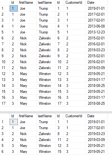
The example shows both INNER JOIN and CROSS APPLY. The INNER JOIN shows everything, but if we want to only show the two newest orders per customer we have to use CROSS APPLY.

A table-valued function could be used instead of a derived table (subquery):

CREATE FUNCTION dbo.GetTwoNewestOrders (@CustomerId INT)
RETURNS TABLE AS
RETURN 
(
  SELECT TOP 2 *
  FROM orders o
  WHERE o.CustomerId = @CustomerId
  ORDER BY Date DESC
)

---

SELECT *
FROM customer c
CROSS APPLY GetTwoNewestOrders(c.Id)

Cursors can sometimes be replaced with the APPLY operator.
CROSS APPLY is called lateral join in PostgreSQL.

OUTER APPLY

OUTER APPLY preserves the left side of in a similar manner as when using LEFT JOIN. Other than that it’s equal to CROSS APPLY.

Query data by using table expressions

Syllabus

Identify basic components of table expressions, define usage differences between table expressions and temporary tables, construct recursive table expressions to meet business requirements

Table expressions

Table expressions are named queries, according to the official exam book. They can also be described as table-valued subqueries. The book also mentions that there are four types of table expressions:

Common table expressions (CTEs)
Views
Derived tables
Inline table-valued functions

Views are explained here. Table-valued functions are explained here. Derived tables are subqueries.

Common table expressions (CTEs)

Official documentation
Introduction to CTEs on Essential SQL

Example of a simple CTE:

WITH customer_order_cte (CustomerId, FirstName, LastName, OrderId, Date) AS
(
SELECT
    c.Id        AS CustomerId
  , c.firstName AS FirstName
  , c.lastName  AS LastName
  , o.Id        AS OrderId
  , o.Date      AS Date
FROM customer c
  INNER JOIN order o ON c.Id = o.CustomerId
)
SELECT *
FROM customer_order_cte

Example of chained CTE:

WITH customer_order_cte (CustomerId, FirstName, LastName, OrderId, Date) AS
(
SELECT
    c.Id        AS CustomerId
  , c.firstName AS FirstName
  , c.lastName  AS LastName
  , o.Id        AS OrderId
  , o.Date      AS Date
FROM customer c
  INNER JOIN order o ON c.Id = o.CustomerId
),
order_order_line_cte (OrderId, Date, OrderLineId, ItemId, Amount) AS
(
SELECT
    o.Id        AS OrderId
  , o.Date      AS Date
  , ol.Id       AS OrderLineId
  , ol.ItemId   AS ItemId
  , ol.Amount   AS Amount
FROM ca_order o
  INNER JOIN order_line ol ON o.Id = ol.OrderId
)
SELECT
    CustomerId
  , FirstName
  , LastName
  , co.OrderId
  , co.Date
  , ItemId
  , Amount
FROM customer_order_cte co
  INNER JOIN order_order_line_cte ool ON co.OrderId = ool.OrderId

INSERT, UPDATE, DELETE and MERGE can also be used in the outer statement of a table expression.

Recursive CTEs

Recursive CTEs on Essential SQL

Recursive CTEs are useful for hierarchical data.

Example:

CREATE TABLE hierarchy (
    Id        INT           IDENTITY(1,1)    NOT NULL
  , Name      VARCHAR(200)
  , ParentId  INT
)

INSERT INTO hierarchy
    (Name          , ParentId) VALUES
    ('Top 1'       , NULL    )
  , ('Middle 1-1'  , 1       )
  , ('Bottom 1-1-1', 2       )
  , ('Bottom 1-1-2', 2       )
  , ('Top 2'       , NULL    )
  , ('Middle 2-1'  , 5       )
  , ('Bottom 2-1-1', 6       )
  , ('Middle 2-2'  , 5       )
  , ('Top 3'       , NULL    )
  , ('Middle 3-1'  , 9       )

----

WITH hierarchy_cte (Id, Name, Level, ParentId, Sort) AS
(
  SELECT
      Id
    , Name
    , 1
    , ParentId
    , CAST (Name AS VARCHAR (200))
  FROM hierarchy
  WHERE ParentId IS NULL

  UNION ALL

  SELECT
      h.Id
    , CAST (REPLICATE('|---', hc.Level) + h.Name AS VARCHAR (200))
    , hc.Level + 1
    , h.ParentId
    , CAST (hc.Sort + '\' + h.Name AS VARCHAR (200))
  FROM hierarchy h
    INNER JOIN hierarchy_cte hc
      ON h.ParentId = hc.Id
)
SELECT
    Name
  , Level
  , ParentId
  , Sort
FROM hierarchy_cte
ORDER BY Sort

Recursive CTE results

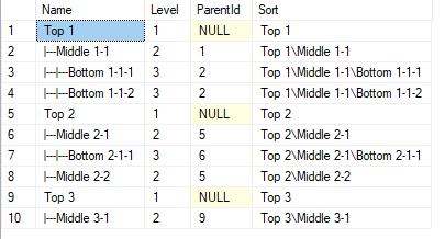
Table expressions vs temporary tables

Temporary tables or table variables should be used when the data is used several times. This is especially true if the data comes from an expensive query. Storing the data in a temporary table or table variable means we don’t have to perform the expensive query several times. Instead, we can read the already queried values from the table, which is much cheaper.

Whether to use a temporary table or table variable depends on the size of the table. For small tables it’s better to use table variables, while large tables should be stored in temporary tables. This is because temporary tables have full statistics, while table variables have very little statistics on them. Small tables don’t need full statistics.

Table expressions are good when the data from the table expression is used only once. Using a table expression means we don’t get the unnecessary overhead that we get when the data is written to the temporary table.

Group and pivot data by using queries

Syllabus

Use windowing functions to group and rank the results of a query; distinguish between using windowing functions and GROUP BY; construct complex GROUP BY clauses using GROUPING SETS, and CUBE; construct PIVOT and UNPIVOT statements to return desired results based on supplied data; determine the impact of NULL values in PIVOT and UNPIVOT queries

GROUP BY

Official documentation on GROUP BY
Official documentation on HAVING

CREATE TABLE people (
    Id          INT           IDENTITY(1,1)    NOT NULL
  , firstName   VARCHAR(200)
  , lastName    VARCHAR(200)
  , age         INT
)

INSERT INTO people (firstName, lastName, age) VALUES
    ('Joe'   , 'Guliani' , 25)
  , ('Aaron' , 'Guliani' , 47)
  , ('Dawn'  , 'Anderson', 55)
  , ('Kilroy', 'Anderson', 52)
  , ('Donald', 'Sanders' , 67)

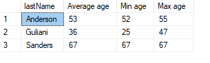
SELECT
    lastName
  , AVG(age) AS 'Average age'
  , MIN(age) AS 'Min age'
  , MAX(age) AS 'Max age'
FROM people
GROUP BY lastName

GROUP BY results

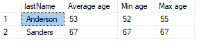
HAVING is used to filter values when using GROUP BY:

SELECT
    lastName
  , AVG(age) AS 'Average age'
  , MIN(age) AS 'Min age'
  , MAX(age) AS 'Max age'
FROM people
GROUP BY lastName
HAVING AVG(age) > 40

GROUP BY with HAVING results

GROUP BY vs windowing functions

Group functions group together rows and then apply the grouping functions to each group. The result is one row per group.

With window functions, a set of underlying rows is defined, and the window function operates on each row.

GROUPING SETS

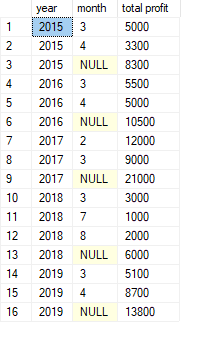
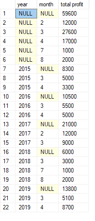
redgate on GROUPING SETS

GROUPING SETS makes multiple combinations of groups to group the data by.

Example:

CREATE TABLE sales (
    Id       INT    IDENTITY(1,1)    NOT NULL
  , year     INT                     NOT NULL
  , month    INT                     NOT NULL
  , profit   INT
)

INSERT INTO sales (year, month, profit) VALUES
    (2015, 03, 2000)
  , (2015, 03, 3000)
  , (2015, 04, 1500)
  , (2015, 04, 1800)
  , (2016, 03, 1000)
  , (2016, 03, 1500)
  , (2016, 03, 3000)
  , (2016, 04, 2000)
  , (2016, 04, 3000)
  , (2017, 02, 7500)
  , (2017, 03, 3000)
  , (2017, 03, 3000)
  , (2017, 03, 3000)
  , (2017, 02, 4500)
  , (2018, 07, 1000)
  , (2018, 08, 2000)
  , (2018, 03, 3000)
  , (2019, 03, 3000)
  , (2019, 03, 2100)
  , (2019, 04, 8700)

SELECT
    year
  , month
  , SUM(profit) AS 'total profit'
FROM sales
GROUP BY GROUPING SETS (
    year
  , (year, month)
  , ()
)

GROUPING SETS results

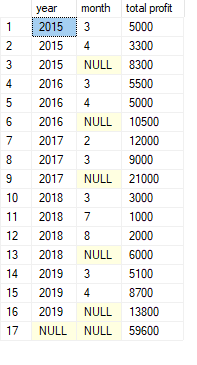
CUBE

CUBE() is a function that generates all the possible grouping sets for us.

Example:

SELECT
    year
  , month
  , SUM(profit) AS 'total profit'
FROM sales
GROUP BY CUBE(year, month)
ORDER BY year, month

CUBE results

ROLLUP

ROLLUP() is a function that generates grouping sets for us. Unlike CUBE(), it doesn’t generate all grouping sets, but rather grouping sets in a hierarchy.

Example:

SELECT
    year
  , month
  , SUM(profit) AS 'total profit'
FROM sales
GROUP BY ROLLUP(year, month)

ROLLUP results

GROUPING and GROUPING_ID

Official documentation on GROUPING
Official documentation on GROUPING_ID
Codingsight on GROUPING and GROUPING_ID

GROUPING() and GROUPING_ID() are used together with GROUP BY.

GROUPING() is used to determine whether a column is aggregated or not.

Example:

SELECT
    year
  , month
  , AVG(profit)       AS 'Average profit'
  , GROUPING(month)   AS 'Grouping (month)'
  , GROUPING(year)    AS 'Grouping (year)'
FROM sales
GROUP BY CUBE (month, year)
ORDER BY GROUPING_ID(month, year)

GROUPING results

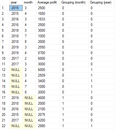
GROUPING() will return 1 if the given column was aggregated and 0 otherwise. From the results above, we can see that the rows were year was aggregated will have NULL in the year cell. This means GROUPING(year) will return 0. The same is true for month were months are aggregated.

GROUPING_ID() calculates the level of grouping. When GROUPING_ID() is used with the same arguments as GROUP BY, it will do the following:

Go through every argument to GROUPING_ID(arg1, arg2, ...) and:
- Calculate GROUPING(arg1). E.g. 1.
- Calculate GROUPING(arg2). E.g. 0.
- etc.
Concatenate the GROUPING() results together. E.g. 10 (binary).
The final value is represented in decimal format. E.g. 3.

Example:

SELECT
    year
  , month
  , AVG(profit)              AS 'Average profit'
  , CAST(GROUPING(month) AS VARCHAR(1)) +
    CAST(GROUPING(year)  AS VARCHAR(1))
                             AS 'GROUPING_ID (binary)'
  , GROUPING_ID(month, year) AS 'GROUPING_ID (decimal)'
FROM sales
GROUP BY CUBE (month, year)
ORDER BY GROUPING_ID(month, year)

GROUPING results

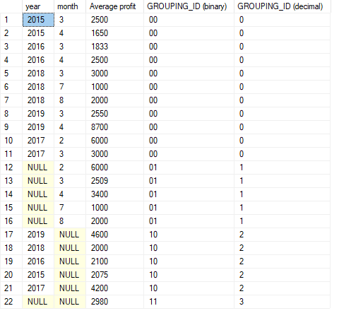
The argument to GROUPING_ID has to be the same as the argument to GROUP BY.

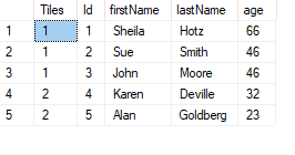
PIVOT and UNPIVOT statements

Official documentation

PIVOT makes rows into columns, and UNPIVOT does the opposite. To make this work, the data has to be grouped and aggregated.

Example:

CREATE TABLE insurances (
    Id             INT         IDENTITY(1,1)   NOT NULL
  , customerId     INT                         NOT NULL
  , policyNo       INT                         NOT NULL
  , insuranceType  VARCHAR(20)                 NOT NULL
)

INSERT INTO insurances (customerId, policyNo, insuranceType) VALUES
    (1, 1234, 'Life')
  , (1, 1235, 'Car')
  , (2, 1236, 'Car')
  , (2, 1237, 'Life')
  , (3, 1238, 'Fire')
  , (4, 1239, 'Liability')
  , (4, 1230, 'Fire')

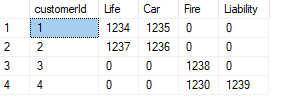
WITH insurancesPivotedCTE AS
(
  SELECT
      customerId        -- grouping column
    , insuranceType     -- spreading column
    , policyNo          -- aggregation column
  FROM insurances
)
SELECT customerId, [Life], [Car], [Fire], [Liability]
FROM insurancesPivotedCTE
  PIVOT (MAX(policyNo) FOR insuranceType  -- aggregate and spreading column
      IN ([Life], [Car], [Fire], [Liability])) AS P

PIVOT results

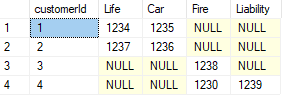
NULL values in PIVOT and UNPIVOT

ISNULL() can be used to change the NULLs into something else.

WITH insurancesPivotedCTE AS
(
  SELECT
      customerId        -- grouping column
    , insuranceType     -- spreading column
    , policyNo          -- aggregation column
  FROM insurances
)
SELECT customerId,
      ISNULL([Life]     , 0) AS Life
    , ISNULL([Car]      , 0) AS Car
    , ISNULL([Fire]     , 0) AS Fire
    , ISNULL([Liability], 0) AS Liability
FROM insurancesPivotedCTE
  PIVOT (MAX(policyNo) FOR insuranceType  -- aggregate and spreading column
      IN ([Life], [Car], [Fire], [Liability])) AS P

PIVOT with ISNULL results

Window functions

Windows functions are only allowed in SELECT or ORDER BY.

Window aggregate functions

Many aggregate functions can also be used as window functions, for example SUM(), MAX(), MIN(), AVG(), COUNT().

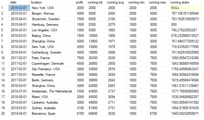
Example:

SELECT
  date
, city + ', ' + country AS location
, profit
, SUM(profit)   OVER(ORDER BY date ROWS UNBOUNDED PRECEDING) AS 'running tot'
, AVG(profit)   OVER(ORDER BY date ROWS UNBOUNDED PRECEDING) AS 'running avg'
, MIN(profit)   OVER(ORDER BY date ROWS UNBOUNDED PRECEDING) AS 'running min'
, MAX(profit)   OVER(ORDER BY date ROWS UNBOUNDED PRECEDING) AS 'running max'
, STDEV(profit) OVER(ORDER BY date ROWS UNBOUNDED PRECEDING) AS 'running stdev'
FROM sales

Window aggregate functions result

Window ranking functions

Official documentation

Ranking functions gives a ranking value for each row in a partition. SQL Server has the following ranking functions: RANK(), DENSE_RANK(), NTILE() and ROW_NUMBER().

RANK() will return the rank of each row within the result set. The rank of one row is the rank of the previous row plus one. RANK() is similar to ROW_NUMBER(), but ROW_NUMBER() numbers rows sequentially, while RANK() provides the same value for ties.
DENSE_RANK is like rank, but doesn’t have any gaps between the ranks.
NTILE() distributes the rows into a given amount of groups.
ROW_NUMBER() numbers rows sequentially.

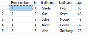
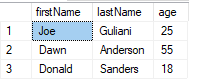
Example using ROW_NUMBER():

SELECT
    ROW_NUMBER() OVER (ORDER BY age DESC) AS 'Row number'
  , *
FROM customers

ROW_NUMBER results

Example using RANK():

SELECT
    RANK() OVER (ORDER BY age DESC) AS 'Rank (oldest)'
  , *
FROM customers

RANK results

Example using DENSE_RANK():

SELECT
    DENSE_RANK() OVER (ORDER BY age DESC) AS 'Dense rank (oldest)'
  , *
FROM customers

DENSE_RANK results

Example using NTILE():

SELECT
    NTILE(2) OVER (ORDER BY age DESC) AS 'Tiles'
  , *
FROM customers

NTILE results

ORDER BY is mandatory.
If the PARTITION clause is missing the entire query result is the partition.
Window ranking functions are non-deterministic and can therefore not be used in indexed views.

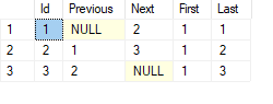
Window offset functions

Official documentation

Window offset functions return values from other rows that are an offset away from the current row in a window partition. LAG(), LEAD(), FIRST_VALUE() and LAST_VALUE() are window offset functions.

LAG() retrieves a value from a previous row in the partition.
LEAD() retrieves a value from a subsequent row in the partition.
FIRST_VALUE() retrieves a value from the first row in the window frame.
LAST_VALUE() retrieves a value from the last row in the window frame. The last row in the window frame is the current row when using a default frame.

LAG() and LEAD() takes an optional offset parameter. Offset is 1 by default.

Example:

SELECT
    Id
  , LAG(Id)         OVER (ORDER BY Id) AS Previous
  , LEAD(Id)        OVER (ORDER BY Id) AS Next
  , FIRST_VALUE(Id) OVER (ORDER BY Id) AS First
  , LAST_VALUE(Id)  OVER (ORDER BY Id) AS Last
FROM customer 

LAG, LEAD, FIRST_VALUE and LAST_VALUE results

Query temporal data and non-relational data

Syllabus

Query historic data by using temporal tables, query and output JSON data, query and output XML data

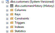
Temporal tables

Official documentation

SQL Server 2016 or later is needed to use temporal tables.

Temporal tables are tables that keep a full history of data changes, rather than just the data at the current time. This makes it possible to retrieve data from any point in the past.

Temporal tables basically consist of a pair of tables: a current table and a history table. Both tables have two columns, in addition to the ordinary data columns, that contain period start and period end. The two period columns are both of DATETIME2 type.

Example:

CREATE TABLE dbo.customers   
(    
    Id          INT           IDENTITY(1,1)   NOT NULL   PRIMARY KEY
  , firstName   VARCHAR(200)
  , lastName    VARCHAR(200)
  , validFrom   DATETIME2 (2) GENERATED ALWAYS AS ROW START  
  , validTo     DATETIME2 (2) GENERATED ALWAYS AS ROW END  
  , PERIOD FOR SYSTEM_TIME (validFrom, validTo)  
 )    
WITH (SYSTEM_VERSIONING = ON (HISTORY_TABLE = dbo.customersHistory));  

System versioned table in SSMS

Temporal tables need a primary key.

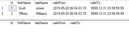
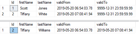
Inserting:

When a row is inserted it gets start time set to the current time in UTC and the end time set to 9999-12-31.

INSERT INTO customers (firstName, lastName) VALUES
    ('Scott'  , 'Jones'   )
  , ('Tiffany', 'Williams')

SELECT * FROM customers
SELECT * FROM customersHistory

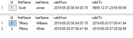
System versioned table after first INSERT

Updating:

When a row is updated, the old value is moved to the history table. The end time in the history table is set to the current time in UTC. The from time in the system-versioned table is set to the current time in UTC.

UPDATE customers SET lastName = 'White' WHERE Id = 2

SELECT * FROM customers
SELECT * FROM customersHistory

System versioned table after first UPDATE

Deleting:

When a row is deleted, it gets moved to the history table. The end time in the history table is set to the current time in UTC. The row is removed from the system-versioned table.

DELETE FROM customers WHERE Id = 2

SELECT * FROM customers
SELECT * FROM customersHistory

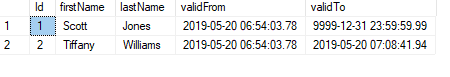
System versioned table after first DELETE

Query:

All values between two datetimes:

SELECT *
FROM customers   
FOR SYSTEM_TIME    
  BETWEEN '2019-05-20 06:00:00.0000000' AND '2019-05-20 08:00:00.0000000'
ORDER BY ValidFrom

Query results with BETWEEN

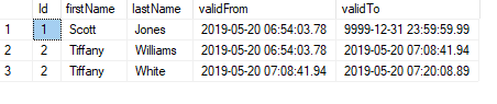
Table at a current date and time:

SELECT *
FROM customers   
FOR SYSTEM_TIME    
  AS OF '2019-05-20 07:00:00.0000000'

Query results with AS OF

To drop a system-versioned table, you must turn off system versioning and drop both the system versioned table and history table.

Example:

ALTER TABLE dbo.customers SET (SYSTEM_VERSIONING = OFF)
DROP TABLE IF EXISTS dbo.customers
DROP TABLE IF EXISTS dbo.customersHistory

XML

Official documentation

XML is a data type in SQL Server. XML can be stored with the XML data type in either untyped format or in typed format. XML columns can be indexed.

XML output

Official documentation

The FOR XML clause is used to output XML. It has four modes:

RAW: Generates a single <row> element per row in the rowset returned by SELECT.
AUTO: Generates nesting in the resulting XML based on how the SELECT is formed.
EXPLICIT: Can be used to generate XML with more control than RAW and AUTO. Can specify whether selected column should be element or attribute. Element and attributes can be mixed.
PATH: Has the flexibility of EXPLICIT, but is easier to use.

XML RAW:

The created XML is close to the relational presentation of data when using XML RAW.

SELECT *
FROM people
FOR XML RAW

<row Id="1" firstName="Joe" lastName="Guliani" age="25" />
<row Id="2" firstName="Aaron" lastName="Guliani" age="17" />
<row Id="3" firstName="Dawn" lastName="Anderson" age="55" />
<row Id="4" firstName="Kilroy" lastName="Anderson" age="5" />
<row Id="5" firstName="Donald" lastName="Sanders" age="18" />

A root node is not added. The result is an XML fragment. FOR XML RAW, ROOT('Customers') can be used to create a root element. The result above uses attributes. To use elements, FOR XML RAW, ELEMENTS should be used instead.

XML AUTO:

SELECT *
FROM people
FOR XML AUTO

<people Id="1" firstName="Joe" lastName="Guliani" age="25" />
<people Id="2" firstName="Aaron" lastName="Guliani" age="17" />
<people Id="3" firstName="Dawn" lastName="Anderson" age="55" />
<people Id="4" firstName="Kilroy" lastName="Anderson" age="5" />
<people Id="5" firstName="Donald" lastName="Sanders" age="18" />

ELEMENTS and ROOT('...') can be used here too.

XML EXPLICIT:

SELECT
    1         AS Tag
  , NULL      AS Parent
  , Id        AS 'Person!1!Id!Element'
  , firstName AS 'Person!1!FirstName'
  , lastName  AS 'Person!1!LastName'
FROM people
FOR XML EXPLICIT

<Person FirstName="Joe" LastName="Guliani">
  <Id>1</Id>
</Person>
<Person FirstName="Aaron" LastName="Guliani">
  <Id>2</Id>
</Person>
<Person FirstName="Dawn" LastName="Anderson">
  <Id>3</Id>
</Person>
<Person FirstName="Kilroy" LastName="Anderson">
  <Id>4</Id>
</Person>
<Person FirstName="Donald" LastName="Sanders">
  <Id>5</Id>
</Person>

XML PATH:

SELECT
    Id        AS '@PersonId'
  , firstName AS 'Name/First'
  , lastName  AS 'Name/Last'
  , age       AS 'Age'
FROM people
FOR XML PATH ('Person')

<Person PersonId="1">
  <Name>
    <First>Joe</First>
    <Last>Guliani</Last>
  </Name>
  <Age>25</Age>
</Person>
<Person PersonId="2">
  <Name>
    <First>Aaron</First>
    <Last>Guliani</Last>
  </Name>
  <Age>17</Age>
</Person>
<Person PersonId="3">
  <Name>
    <First>Dawn</First>
    <Last>Anderson</Last>
  </Name>
  <Age>55</Age>
</Person>
<Person PersonId="4">
  <Name>
    <First>Kilroy</First>
    <Last>Anderson</Last>
  </Name>
  <Age>5</Age>
</Person>
<Person PersonId="5">
  <Name>
    <First>Donald</First>
    <Last>Sanders</Last>
  </Name>
  <Age>18</Age>
</Person>

XML parsing

Official documentation

OPENXML can be used to parse XML and return the values as rows and columns. sp_xml_preparedocument is used to prepare the XML for parsing. sp_xml_removedocument must be used after parsing the XML. Preparing is not needed when the XML is typed.

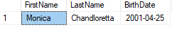
Example with single element containing sub elements:

DECLARE @xml VARCHAR(MAX) = 
'<?xml version="1.0" encoding="UTF-8"?>
<Person>
  <FirstName>Monica</FirstName>
  <LastName>Chandloretta</LastName>
  <BirthDate>2001-04-25</BirthDate>
</Person>'

DECLARE @preppedXmlHandle INT

EXEC sp_xml_preparedocument @preppedXmlHandle OUTPUT, @xml; 

SELECT *
FROM OPENXML(@preppedXmlHandle, '/Person', 2)
  WITH (
        FirstName  VARCHAR(200)
      , LastName   VARCHAR(200)
      , BirthDate  DATE
    )

EXEC sp_xml_removedocument @preppedXmlHandle

OPENXML results

Example with two elements containing attributes:

DECLARE @xml VARCHAR(MAX) = 
'<?xml version="1.0" encoding="UTF-8"?>
<People>
  <Person FirstName="Monica"   LastName="Chandloretta" BirthDate="2001-04-25"/>
  <Person FirstName="Chandler" LastName="Moniquer"     BirthDate="1995-08-02"/>
</People>'

DECLARE @preppedXmlHandle INT

EXEC sp_xml_preparedocument @preppedXmlHandle OUTPUT, @xml; 

SELECT *
FROM OPENXML(@preppedXmlHandle, '/People/Person', 1)
  WITH (
        FirstName  VARCHAR(200)
      , LastName   VARCHAR(200)
      , BirthDate  DATE
    )

EXEC sp_xml_removedocument @preppedXmlHandle

OPENXML with attributes results

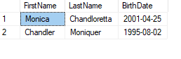
The second argument to OPENXML() specifies whether the parsing should be element-centric or attribute-centric:
- 1: attribute-centric
- 2: element-centric

XML querying

Official documentation

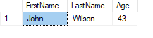
value() can be used to get values in the XML.

Example:

DECLARE @xml XML =
'<People>
  <Person FirstName="John"   LastName="Wilson"   Age="43"/>
  <Person FirstName="Lauren" LastName="Adeleres" Age="52"/>
</People>'

SELECT
    @xml.value('(/People/Person/@FirstName)[1]', 'VARCHAR(200)') AS FirstName
  , @xml.value('(/People/Person/@LastName)[1]' , 'VARCHAR(200)') AS LastName
  , @xml.value('(/People/Person/@Age)[1]'      , 'INT'         ) AS Age

Results from value

Instead of getting a value like value() does, nodes() can will get a reference to the selected node. This reference can be used for additional queries.

Example:

DECLARE @xml XML =
'<People>
  <Person FirstName="John"   LastName="Wilson"   Age="43"/>
  <Person FirstName="Lauren" LastName="Adeleres" Age="52"/>
</People>'

SELECT
  X.root.value('(/People/Person/@FirstName)[1]', 'VARCHAR(200)') AS firstName  
FROM @xml.nodes('/') AS X(root)

-- output is 'John'

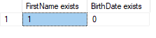
exist() can be used to determine whether an element or attribute exists.

Example:

DECLARE @xml XML =
'<People>
  <Person FirstName="John"   LastName="Wilson"   Age="43"/>
  <Person FirstName="Lauren" LastName="Adeleres" Age="52"/>
</People>'

SELECT
    @xml.exist('(/People/Person/@FirstName)[1]') AS 'FirstName exists'
  , @xml.exist('(/People/Person/@BirthDate)[1]') AS 'BirthDate exists'

Results from exist

modify() is used to modify the XML.

Example:

DECLARE @xml XML =
'<People>
  <Person FirstName="John"   LastName="Wilson"   Age="43"/>
  <Person FirstName="Lauren" LastName="Adeleres" Age="52"/>
</People>'

SELECT @xml

/* Output:
<People>
  <Person FirstName="John"   LastName="Wilson"   Age="43" />
  <Person FirstName="Lauren" LastName="Adeleres" Age="52" />
</People>
*/

SET @xml.modify(
  'replace value of (/People/Person/@FirstName)[1]
   with "Jonathan"')

SET @xml.modify(
  'insert <Person FirstName="Ashley" LastName="Saxon" Age="15"/>
   as last into (/People)[1]')

SET @xml.modify('delete (/People/Person)[2]')

SELECT @xml

/* Output:
<People>
  <Person FirstName="Jonathan" LastName="Wilson" Age="43" />
  <Person FirstName="Ashley"   LastName="Saxon"  Age="15" />
</People>
*/

query() is used to query the content in the XML.

Example:

DECLARE @xml XML =
'<People>
  <Person FirstName="John"   LastName="Wilson"   Age="43"/>
  <Person FirstName="Lauren" LastName="Adeleres" Age="52"/>
</People>'

SELECT @xml.query('/People/Person[@FirstName="John"]')

-- Output: <Person FirstName="John" LastName="Wilson" Age="43" />

SELECT @xml.query('/People/Person[@Age>50]')

-- Output: <Person FirstName="Lauren" LastName="Adeleres" Age="52" />

JSON

Official documentation

SQL Server does not support a native JSON data type. VARCHAR is usually used instead.

This variable with JSON in it is used in many of the examples:

DECLARE @json VARCHAR(MAX) =
'{
  "firstName": "Pete",
  "lastName": "Carpenter",
  "age": 56
}'

JSON output

Example of FOR JSON PATH:

-- customers table from examples above
SELECT *
FROM customers
FOR JSON PATH

Prints:

[
  {
    "Id": 1,
    "firstName": "John",
    "lastName": "Smith",
    "age": 46
  },
  {
    "Id": 2,
    "firstName": "Joe",
    "lastName": "Schmoe",
    "age": 12
  },
  {
    "Id": 3,
    "firstName": "Mary",
    "lastName": "Christ",
    "age": 74
  }
]

JSON parsing

Official documentation

OPENJSON() can be used to parse JSON and return the values as rows and columns.

Example:

SELECT *
FROM OPENJSON(@json)
WITH (
  firstName VARCHAR(50),
  lastName  VARCHAR(100),
  age       INT
)

OPENJSON output

JSON querying

To check whether a string is valid JSON, use ISJSON(). To read a scalar value, use JSON_VALUE().

PRINT ISJSON(@json)    -- Outputs 1

PRINT JSON_VALUE(@json, '$.firstName')  -- Outputs 'Pete'

To modify the JSON, use JSON_MODIFY():

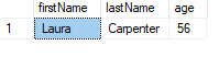
SET @json = JSON_MODIFY(@json, '$.firstName', 'Laura')

PRINT @json

This would output:

{
  "firstName": "Laura",
  "lastName": "Carpenter",
  "age": 56
}

JSON_QUERY() is used to get values for objects and arrays. For scalar values, use JSON_VALUE().

Example:

DECLARE @json VARCHAR(MAX) =
'{
  "name": {
    "firstName": "Pete",
      "lastName": "Carpenter"
  },
  "age": 56
}'

SELECT JSON_QUERY(@json, '$.name')

This would output:

{
  "firstName": "Pete",
  "lastName": "Carpenter"
}

Program databases by using Transact-SQL (25–30%)

Create database programmability objects by using Transact-SQL

Syllabus

Create stored procedures, table-valued and scalar-valued user-defined functions, triggers, and views; implement input and output parameters in stored procedures; identify whether to use scalar-valued or table-valued functions; distinguish between deterministic and non-deterministic functions; create indexed views

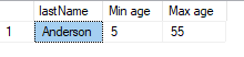
Stored procedures

Official documentation

Example:

CREATE PROCEDURE GetMinAndMaxAgeForLastName
  @lastName VARCHAR(200)
AS
BEGIN
  SET NOCOUNT ON;

  SELECT
      lastName
    , MIN(age) AS 'Min age'
    , MAX(age) AS 'Max age'
  FROM people
  WHERE lastName = @lastName
  GROUP BY lastName
END

Usage:

EXEC GetMinAndMaxAgeForLastName 'Anderson'

Stored procedure results

Stored procedures cannot be used in queries.
Stored procedures can only return an integer return code. Usually to indicate success or failure. 0 usually indicates success, and anything else indicates failure.

Table-valued user-defined function

Table-valued user-defined functions return a table. There are two different types of table-valued functions: inline and multi-statement.

Inline table-valued functions have better performance than multi-statement table-valued functions, because SQL Server will calculate the execution plans of the inline table-valued functions with the latest statistics. This does not happen with multi-statement table-valued functions. More on that here.

Inline table-valued functions:

Are similar to views because it’s a single query. Unlike views, it supports parameters.

Example:

CREATE FUNCTION GetCustomersWithLastName (@lastName VARCHAR(100))
RETURNS TABLE AS
    RETURN
        SELECT *
        FROM customers
        WHERE lastName = @lastName

Usage:

SELECT *
FROM GetCustomersWithLastName('Smith')

The return statement is simply RETURNS TABLE.
The body does not need BEGIN or END, because it consists of a single query.

Multi-statement table-valued functions:

Very similar to inline table-valued functions, but support multiple statements, as the name suggests.

Example:

CREATE FUNCTION GetMostProfitableSales (@amount INT)
RETURNS 
@sales TABLE 
(
    Id     INT    NOT NULL
  , year   INT    NOT NULL
  , month  INT    NOT NULL
  , profit INT
)
AS
BEGIN
  INSERT INTO @sales
  SELECT TOP (@amount) *
  FROM sales
  ORDER BY Profit DESC
  
  RETURN 
END

Usage:

SELECT * FROM GetMostProfitableSales(3)

The return statements must contain a definition of the output table.
BEGIN and END are needed, because there are multiple statements in the function body.

Scalar-valued user-defined function

Scalar-valued user-defined functions return one value.

Example:

CREATE FUNCTION GetBirthMonthFromSSN (@SSN VARCHAR(11))
RETURNS INT AS
BEGIN
    DECLARE @BirthMonth INT
    SET @BirthMonth = CAST(SUBSTRING(@SSN, 3, 2) AS INT)

    RETURN @BirthMonth
END

Usage:

DECLARE @BirthMonth INT

EXEC @BirthMonth = dbo.GetBirthMonthFromSSN '24119812345'

PRINT @BirthMonth   -- prints 11

Functions in general

User-defined functions can be used in queries.
Must return a value.
Cannot use PRINT or SELECT inside them.
Can have schema bindings.

Triggers

Official documentation

Triggers are special stored procedures that are connected to tables. Triggers can be set to fire when INSERT, UPDATE, DELETE and similar statements are used on a table. Triggers are often used to maintain the integrity of the table.

Triggers use virtual tables that are called inserted and deleted. The rows that are supposed to be deleted or inserted are put in these tables first. The trigger will then act on these tables to check whether the rows should be inserted/deleted or not.

Triggers should not be used for ordinary integrity checks. Native constraints (check constraint, uniqueness, etc.) should be used instead. This is because triggers have a performance overhead.

Types of triggers:

AFTER: starts after the execution that fired the trigger. After constraints. Will not be fired if the execution failed.
INSTEAD OF: starts before the execution that fired the trigger.
CLR triggers: written in .NET languages. Not part of the syllabus.
Logon triggers: run when a user session is established. Not part of the syllabus.

Example:

CREATE TRIGGER dbo.accounts_trgi ON dbo.accounts AFTER INSERT
AS
BEGIN
  SET NOCOUNT ON

  IF EXISTS(SELECT 1 FROM inserted WHERE firstName = '' OR lastName = '')
  BEGIN
    RAISERROR('The first name or last name cannot be blank.', 16, 1)
    ROLLBACK TRAN
    RETURN
  END

  IF EXISTS(SELECT 1 FROM inserted i INNER JOIN accounts a ON a.SSN = i.SSN)
  BEGIN
    RAISERROR('Person already exists with that SSN.', 16, 1)
    ROLLBACK TRAN
    RETURN
  END
END

GO

ALTER TABLE dbo.accounts ENABLE TRIGGER accounts_trgi

Views

Official-documentation

Views are premade queries.

Example:

CREATE TABLE people (
    Id           INT            IDENTITY(1,1)    NOT NULL
  , firstName    VARCHAR(200)
  , lastName     VARCHAR(200)
  , age          INT
)

INSERT INTO people (firstName, lastName, age) VALUES
    ('Joe'   , 'Guliani' , 25)
  , ('Aaron' , 'Guliani' , 17)
  , ('Dawn'  , 'Anderson', 55)
  , ('Kilroy', 'Anderson', 5)
  , ('Donald', 'Sanders' , 18)

CREATE VIEW OveragePeople
AS
  SELECT *
  FROM people
  WHERE 18 <= age

SELECT *
FROM OveragePeople

View results

Restrictions:

1024 columns
Single query
Single table when using INSERT
Restricted data modifications
No TOP without ORDER BY
No ORDER BY without TOP, OFFSET or FOR XML.

These options can be added to the view:

WITH SCHEMABINDING: No changes to underlying table.
WITH ENCRYPTION: Encrypts the view.
WITH CHECK: Cannot do updates that removes the updated rows from the view.

Indexed views

Official documentation

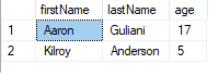
CREATE VIEW UnderagePeople
WITH SCHEMABINDING
AS
  SELECT
      firstName
    , lastName
    , age
  FROM dbo.people
  WHERE age < 18

CREATE UNIQUE CLUSTERED INDEX IX_lastName 
ON dbo.UnderagePeople(firstName, lastName)

SELECT *
FROM UnderagePeople

Indexed view results

Needs WITH SCHEMABINDING.
Schema name is needed in the table used in FROM.
Cannot use non-deterministic functions in the view.
Cannot use functions that returns values with FLOAT type.
When the view is schema bound you cannot use SELECT *.

Implement error handling and transactions

Syllabus

Determine results of Data Definition Language (DDL) statements based on transaction control statements, implement TRY…CATCH error handling with Transact-SQL, generate error messages with THROW and RAISERROR, implement transaction control in conjunction with error handling in stored procedures

Transaction control

A transaction is a unit of work. Transactions are used to get the following properties:

Atomicity: everything happens, or nothing happens.
Consistency: the database should transition to one consistent state to another.
Isolation: intermediate states are only visible to the transaction.
Durability: a committed transaction will survive permanently.

A transaction is made explicitly with BEGIN TRANSACTION and committed with COMMIT TRANSACTION or rolled back with ROLLBACK TRANSACTION. TRAN can be used instead of TRANSACTION. Explicitly made transactions are called user-defined transactions. There also implicitly made transactions called system-made transactions. There are even implicitly user-defined transactions, but these are rarely used.

Example:

BEGIN TRAN

SELECT * FROM customers -- empty table, so no rows

INSERT INTO customers VALUES ('Trevor', 'Tate')

ROLLBACK TRAN

SELECT * FROM customers -- empty table

Results when rolled back transaction

The transaction was rolled back, so the customers table is still empty.

Example:

BEGIN TRAN

SELECT * FROM customers

INSERT INTO customers VALUES ('Trevor', 'Tate')

COMMIT TRAN

SELECT * FROM customers

Results when committed transaction

Because the transaction was committed it will have the Trevor Tate customer.

SET XACT_ABORT ON can be used to get more consistent behavior when an error occurs in the transaction. When it’s on and an error occurs, the execution of code is aborted, and the transaction is rolled back automatically.

@@TRANCOUNT returns a number. It will increment when BEGIN TRANSACTION runs and decrement when COMMIT is run. ROLLBACK TRANSACTION (except with a savepoint) will set @@TRANCOUNT to 0. @@TRANCOUNT can therefore be used to check if we are in an open transaction.

XACT_STATE() can also be used to check the status of a transaction. It returns:

0 when no transaction is open.
1 when the transaction is open and committable.
-1 when the transaction is doomed.

TRY-CATCH

Official documentation
Erland Sommerskog on error handling

TRY-CATCH is used to handle errors in SQL Server. Place ordinary code within the TRY block and error handling in the CATCH block. If no errors are thrown, the CATCH block is never activated.

Example:

CREATE TABLE customers (
    Id        INT           IDENTITY(1,1)  NOT NULL
  , firstName VARCHAR(200)
  , lastName  VARCHAR(200)
  , age       INT
  , CONSTRAINT CK_age CHECK (age BETWEEN 18 and 80)
)

BEGIN TRY
  INSERT INTO dbo.customers (firstName, lastName, age) VALUES
      ('John'  , 'Smith'   , 120)
    , ('Anette', 'DeLorean', 43 )
END TRY
BEGIN CATCH
  PRINT 'In CATCH'
  PRINT 'Error message: ' + ERROR_MESSAGE()
END CATCH

/* Output:
In CATCH
Error message: The INSERT statement conflicted with the CHECK constraint
"CK_age". The conflict occurred in database "test", table "dbo.customers",
column 'age'.
*/

TRY-CATCH can be nested. For example, a new nested TRY-CATCH inside the first CATCH.
If TRY-CATCH isn’t used the error will bubble up the call stack. If there are no TRY-CATCH statements the caller will receive an error.
If a new error happens inside the CATCH block, and it isn’t wrapped in a new TRY-CATCH, it will bubble up.
Compilation errors are not transferred to the CATCH block in the same scope they occur in.
TRY-CATCH is not allowed in user-defined functions.

Error functions

SQL Server has the following functions that provide information about an error that has been thrown:

ERROR_NUMBER(): returns the error number of the error.
ERROR_MESSAGE(): returns the message text of the error.
ERROR_SEVERITY(): returns the severity value of the error.
ERROR_STATE(): returns the state number of the error.
ERROR_LINE(): returns the line number of occurrence of an error.
ERROR_PROCEDURE(): returns the name of the stored procedure or trigger where an error occurs.

Note:

They must all be used within a CATCH block.
Error functions return NULL outside a CATCH block.
Error functions return info about the innermost CATCH block, if there are several nested CATCH blocks.

THROW

THROW raises an error.

Example:

;THROW 50000, 'Error message', 1

The first parameter is the error number, the second is the error message and the third is a state variable. The error number must be 50000 or larger. State are between 1 and 255 and are used for informational purposes.

Or without parameters:

;THROW

This rethrows the original error.

If the throw happens outside a TRY block it will abort the batch. If it’s inside it will activate the CATCH block.

THROW always uses severity level 16.

RAISERROR

RAISERROR() is older, but has more options, than THROW.

Example:

RAISERROR('Error message', 16, 1)

The first parameter is the error message, the second is the severity and the third is a state variable. Severity determines how the system should behave towards the error:

0 to 10 are informational and are only printed.
11 to 19 are errors that can be caught.
20 to 25 terminates the connection.

State are between 1 and 255 and are used for informational purposes.

There is also a variant with printf-style syntax:

RAISERROR('Error message: %s, %s', 16, 1, 'test1', 'test2')

There two extra options that can be added to RAISERROR():

WITH NOWAIT: used to raise the error immediately, rather than wait until the buffer is full.
WITH LOG: logs the error in the error and application log, and required for severity 19 and up.

Example:

RAISERROR('Error message', 16, 1) WITH NOWAIT
RAISERROR('Error message', 22, 1) WITH LOG

RAISERROR is usually used with severity level 16.
PRINT is a stripped-down version of RAISERROR. PRINT always uses severity level 0.

THROW vs RAISERROR

The official exam book has this table that compares THROW against RAISERROR:

Property	`THROW`	`RAISERROR`
Can re-throw original system error	Yes	No
Activates `CATCH` block	Yes	Yes, when 10 < severity < 20
Always aborts batch when not using `TRY-CATCH`	Yes	No
Aborts/dooms transaction if `XACT_ABORT` is off	No	No
Aborts/dooms transaction if `XACT_ABORT` is on	Yes	No
If error number is passed, it must be defined in `sys.messages`	No	Yes
Supports printf parameter markers directly	No	Yes
Supports indicating severity	No	Yes
Supports `WITH LOG` to log error to error log and application log	No	Yes
Supports `WITH NOWAIT` to send messages immediately to the client	No	Yes
Preceding statements needs to be terminated	Yes	No

Implement data types and NULLs

Syllabus

Evaluate results of data type conversions, determine proper data types for given data elements or table columns, identify locations of implicit data type conversions in queries, determine the correct results of joins and functions in the presence of NULL values, identify proper usage of ISNULL and COALESCE functions

Proper data types for elements and columns

SQL Server supports several data types in various categories:

Exact numeric: INT, NUMERIC.
Character string: CHAR, VARCHAR.
Unicode character string: NCHAR, NVARCHAR.
Approximate numeric: FLOAT, REAL.
Binary strings: BINARY, VARBINARY.
Date and time: DATE, TIME, SMALLDATETIME, DATETIME, DATETIME2, DATETIMEOFFSET.
Boolean: BIT.

Important things to take into account when choosing a data type:

The data type should represent the model.
Data types acts as constraints. A proper date type should be chosen to enforce integrity in the database. E.g. an integer cannot be stored in a VARCHAR, and a character string can not be stored in an INT.
The size of the data type is important. If an attribute can vary between 0 and 100, a TINYINT should be used over INT, as TINYINT only needs 1 byte whereas INT requires 4 bytes. The smallest data type that suits our needs, in the long run, should be used.
FLOAT and REAL are only approximate. If a value has to be represented with preciseness then, an exact numeric type should be used.
When CHAR(X) is used, it will always use a storage of X characters, even if less characters are specified. While this may take more space than a VARCHAR(20), it makes updates faster.
When VARCHAR(Y) is used, it will use less storage than CHAR(Y), because VARCHAR only stores the characters that are specified. Less storage used means better read performance.
CHAR and VARCHAR uses 1 byte per character and only supports one language besides English. NCHAR and NVARCHAR uses 2 bytes per character and can use Unicode.
NOT NULL should be used to disallow NULL in variables that should never be NULL.

Data type conversions

Official documentation on data type precedence

Literals must be on the correct form.

Type	Literal
`VARCHAR`	`'This is a varchar'`
`NVARCHAR`	`N'This is an nvarchar'`
`INT`	`1`
`FLOAT`	`1.1`
`REAL`	`1.1`
`DECIMAL`	`1.1`
`DATE`	`'2018-05-18'`

Casting NUMERIC to INT truncates the value:

SELECT CAST(1.99999 AS INT)     -- output is 1

Converting a NUMERIC of higher scale to a NUMERIC with lower scale rounds the number:

SELECT CAST(1.99999 AS NUMERIC(3, 2)) -- output is 2.00.

When converting a string with datetime to a DATETIME you get rounding:

DECLARE @dt DATETIME = '2019-05-18 12:55:00.999'

SELECT @dt  -- output is 2019-05-18 12:55:01.000

When converting a datetime type of a higher precision to one with less precision, you get rounding:

DECLARE @dt2 DATETIME2 = '2019-05-18 12:55:00.9999999'

SELECT
    @dt2                    -- output is 2019-05-18 12:55:00.9999999
  , CAST(@dt2 AS DATETIME)  -- output is 2019-05-18 12:55:01.000

Locations of implicit data type conversions in queries

When an expression involves different types, SQL Server will implicitly convert the various types when that’s possible. Explicit conversions; using CAST, CONVERT, etc.; can be beneficial.

SQL Server usually converts the types with lower precedence to the ones with higher precedence.

Example:

SELECT 2 + '2'

Outputs 4, because INT has higher precedence than VARCHAR.

If all operands in an expression are of the same type, the result will be of that type.

Example:

SELECT 11 / 2     -- output is 5

Because 11 and 2 are INTs, the output will be an INT as well. Because FLOAT and REAL have higher precedence than INT, the following will output 5.5:

SELECT 11.0 / 2   -- output is 5.500000

Because 2 will be implicitly converted to 2.0.

CAST(col AS NUMERIC(10, 3)) can be used if the operands are columns or variables:

DECLARE @dividend INT = 11
DECLARE @divisor  INT = 2

SELECT CAST(@dividend AS NUMERIC(10, 3)) /
       CAST(@divisor  AS NUMERIC(10, 3))   -- output is 5.50000000000000

Correct results when joins and NULL values

See section Query multiple tables by using joins.

ISNULL()

Returns the first value that is not NULL. Supports two parameters.

Example:

DECLARE @a INT = NULL
DECLARE @b INT = 1

SELECT ISNULL(@a, @b)   -- outputs 1

ISNULL() is T-SQL and not part of the SQL standard.

COALESCE()

Returns the first value that is not NULL. Supports more than two parameters.

Example:

DECLARE @a INT = NULL
DECLARE @b INT = NULL
DECLARE @c INT = 2

SELECT COALESCE(@a, @b, @c)   -- outputs 2

COALESCE() is part of the SQL standard.

ISNULL() vs COALESCE()

The official exam book has a nice table that summarizes the differences between ISNULL() and COALESCE():

Property	`ISNULL()`	`COALESCE()`
Parameters	2	> 2
SQL standard	no	yes
Data type of result	1. If first input has type, then that type. 2. Else, if second input has type, then that type. 3. If both inputs are untyped NULLs, then INT.	1. If at least one input has type, then type with highest precedence. 2. If all inputs are untyped NULLs, then error.
Nullability of result	If any input is non-nullable, the result is NOT NULL, otherwise NULL.	If all inputs are non-nullable, the result is NOT NULL, otherwise NULL.
Might execute sub query more than once	no	yes

Not part of the official syllabus

The things in this chapter is not part of the official syllabus but should be known about anyway. I don’t know if spatial data types will show up on the exam, but cursors will for sure.

Spatial data

redgate on spatial data

Geography

Official documentation

geography is a data type in SQL Server that stores longitude and latitude.

Example:

CREATE TABLE customers   
(
    Id                 INT            IDENTITY (1,1)  NOT NULL
  , firstName          VARCHAR(200)
  , lastName           VARCHAR(200)
  , customer_location  geography
)

INSERT INTO customers (firstName, lastName, customer_location) VALUES
    ('Jon' , 'Snow' , geography::Parse('POINT(5.0 60.0)'))
  , ('Arya', 'Stark', geography::Parse('POINT(4.0 58.0)'))

Geometry

Official documentation

geometry is a data type in SQL Server that stores spatial data in a flat coordinate system.

Example:

CREATE TABLE employees   
(
    Id                 INT            IDENTITY (1,1)  NOT NULL
  , firstName          VARCHAR(200)
  , lastName           VARCHAR(200)
  , desk_location      geometry
)

INSERT INTO employees (firstName, lastName, desk_location) VALUES
    ('Jon' , 'Snow' , geometry::Parse('POINT(44 27 0)'))
  , ('Arya', 'Stark', geometry::Parse('POINT(44 15 1)'))

SELECT
    firstName + ' ' + lastName AS Name
  , desk_location.STX AS X
  , desk_location.STY AS Y
  , desk_location.Z   AS Z
FROM employees

Geography vs geometry

geography uses a round-earth coordinate system.
geometry uses a flat coordinate system.

Cursors

A control structure that enables traversal over the records in a database.
Like an iterator in programming languages.
A pointer to one row in a set of rows.
Remember DOFCD:
- Declare
- Open
- Fetch next row
- Close
- Deallocate

Example:

DECLARE @Name VARCHAR(40)

DECLARE cursor_test CURSOR FOR
  SELECT TOP 10 Name FROM accounts

OPEN cursor_test

FETCH NEXT FROM cursor_test INTO @Name

WHILE @@FETCH_STATUS = 0  
BEGIN   
  PRINT @Name

  FETCH NEXT FROM cursor_test INTO @Name
END

CLOSE cursor_test
DEALLOCATE cursor_test

UPDATE <table> WHERE CURRENT OF <cursor> can be used to update the row the cursor is at.

Example:

DECLARE @lastName  VARCHAR(200)

DECLARE MyCursor CURSOR FOR
  SELECT lastName FROM customers

OPEN MyCursor

FETCH NEXT FROM MyCursor INTO @lastName

WHILE @@FETCH_STATUS = 0  
BEGIN
  IF @lastName IS NULL
    UPDATE customers SET lastName = 'To delete'
    WHERE CURRENT OF MyCursor

  FETCH NEXT FROM MyCursor INTO @lastName
END

CLOSE MyCursor
DEALLOCATE MyCursor

DELETE <table> WHERE CURRENT OF <cursor> can be used to delete the row the cursor is at.

Example:

DECLARE @lastName  VARCHAR(200)

DECLARE MyCursor CURSOR FOR
  SELECT lastName FROM customers

OPEN MyCursor

FETCH NEXT FROM MyCursor INTO @lastName

WHILE @@FETCH_STATUS = 0  
BEGIN
  IF @lastName IS NULL
    DELETE customers WHERE CURRENT OF MyCursor

  FETCH NEXT FROM MyCursor INTO @lastName
END

CLOSE MyCursor
DEALLOCATE MyCursor

Table of Contents

Manage data with Transact-SQL (40–45%)

Create Transact-SQL SELECT queries

Syllabus

SELECT in general

UNION and UNION ALL

Difference between UNION and UNION ALL

INTERSECT

EXCEPT

Special rules

Query multiple tables by using joins

Syllabus

Joins

INNER JOIN

LEFT JOIN

RIGHT JOIN

FULL OUTER JOIN

CROSS JOIN

Query with NULL on joins

Implement functions and aggregate data

Syllabus

Scalar-valued functions

Table-valued functions

WHERE clause sargability

Differences between deterministic and non-deterministic functions

Type conversion functions

Built-in aggregate functions

Arithmetic functions

Character functions

Date-related functions

Case expressions

System functions

Modify data

Syllabus

INSERT

UPDATE

DELETE

MERGE

OUTPUT

Query data with advanced Transact-SQL components (30–35%)

Query data by using subqueries and APPLY

Syllabus

Subqueries

Subqueries vs joins

CROSS APPLY

OUTER APPLY

Query data by using table expressions

Syllabus

Table expressions

Common table expressions (CTEs)

Recursive CTEs

Table expressions vs temporary tables

Group and pivot data by using queries

Syllabus

GROUP BY

GROUP BY vs windowing functions

GROUPING SETS

CUBE

ROLLUP

GROUPING and GROUPING_ID

PIVOT and UNPIVOT statements

NULL values in PIVOT and UNPIVOT

Window functions

Query temporal data and non-relational data

Syllabus

Temporal tables

XML

XML output

XML parsing

XML querying

JSON

JSON output

JSON parsing

JSON querying

Program databases by using Transact-SQL (25–30%)

Create database programmability objects by using Transact-SQL

Syllabus

Stored procedures

Table-valued user-defined function

Scalar-valued user-defined function